General steps/checks to go through for a reasonable RMC fitting
1. Reciprocal space
In RMCProfile, we follow the convention of defining symbols for various functions as presented in section-2 of Ref. [1]. It is always strongly recommended that before feeding the data into RMCProfile, we should check the format of the data to see whether it is consistent with what we specify in the input for RMCProfile. For example, in our RMCProfile control file we specify our data format to be ‘F(Q)’, that means we are referring our data to be the same format as defined by Eqn. (14) in Ref. [1]. It is noteworthy that in the community, people use the same symbol ‘F(Q)’ to represent another format of the reciprocal space data, which is something like ‘Q[S(Q)-1]’, where S(Q) is the normalized total scattering structure factor as quoted in Eqn. (19-21) in Ref. [1]. To tell which version of the data that the symbol ‘F(Q)’ is representing, we can plot the data and inspect the low-Q region – if it is following our RMCProfile definition, the low-Q level should be somewhat sitting on a flat level (though, in practice it may not be purely flat due to low-Q noise). If it is following the ‘Q[S(Q)-1]’ definition, the low-Q level should then be sitting on an obvious slope due to the multiplicative Q term in the definition.
2. Real space
Similarly in real space, we also need to pay attention to the representation of the same symbol used in the community for different definitions. Again, in RMCProfile, we follow the definition as given in section-2 in Ref. [1]. For example, when we say our data is in ‘G(r)’ format, we mean Eqn. (10) in Ref. [1]. The asymptotic behavior at low-r and high-r region is accordingly presented in Eqn. (15) in Ref. [1]. Sometimes, with the same symbol ‘G(r)’, one may mean the definition as in Eqn. (43) in Ref. [1], e.g., in PDFgui community. The way to tell which version we mean by ‘G(r)’ is similar as above – we plot the data and inspect the low-r region. If we see our data is sitting on an obvious slope, that mean we have the definition as in PDFgui community. Otherwise, if the level at low-r is somewhat flat, we are following the RMCProfile definition. As always, we need to do the necessary homeword to check the data before throwing it into RMCProfile. The fitting engine will take what we tell it as granted and do whatever it can do to fit the data. So, if we tell it something wrong, it can never do it right.
Following the definition of discrete Fourier transform (see Wikipedia, for example), we require the data to be transformed sitting on an equally-spaced grid. If our original data is not in such format, we could use the tool rebin that is bundled in RMCProfile release package to rebin the data to be equally-space. Usage of this tool is straightforward – just input the starting and ending points together with the interval following the order as prompted on terminal, it should do the job properly.
Quite often, the data we hold in hand is not in the absolute scale. By that, we mean if we follow the standard definition to process our raw data to arrive at a certain format of total scattering data and we take the reduced data as the target of our theoretical modeling (using either RMCProfile or whatever other methods), we do not expect an extra fator to compensate the scale difference between our model and data. Dealing with data not on an absolute scale may not be an issue for unit-cell based approach since the scale factor can be taken as one of the refinable parameters among other limited number of parameters. However, for RMC approach with huge number of degree of freedoms, it is always beneficial if we can possibly bring the data to the absolute scale.
To do that, we can use the stog_new tool bundled in RMCProfile release package. Here follows we have a template input for this tool (comments here are for instruction purpose only – in pratice when running stog_new, comments are not allowed),
1 # Number of files
input_binned_data.dat # Input file name
0.4 30.0 # Qmin Qmax
0 1 # yoffset yscale, so that output_y = data/yscale + yoffset
0 # Qoffset, normally we can leave it as 0
scale.sq # scaled S(Q)
scale.gr # scaled G(r)
50 # rmax
5000 # Number of points in r-space
N # windows function? (which makes the peaks more smooth, less noise, less ripples)
0.0764 # number density (angstrom^-3)
0 # yoffset, normally we can keep it as 0
N # Try again, normally keep it as 'N'
Y # Fourier Filter?
1.0 # rcutoff for Fourier filter, meaning data in real-space below the
# cutoff will be filtered out. The corresponding components will also be
# removed in Q-space
scale_ft.sq # Fourier filtered S(Q)
scale_ft.gr # Fourier filtered G(r)
0.08 # Faber-Ziman coefficient, for X-ray, we can put 1 here.
scale_ft_rmc.fq # F(Q) used by RMC
scale_ft_rmc.gr # G(r) used by RMC
scale_ft_rmc.dr # D(r) used by RMC
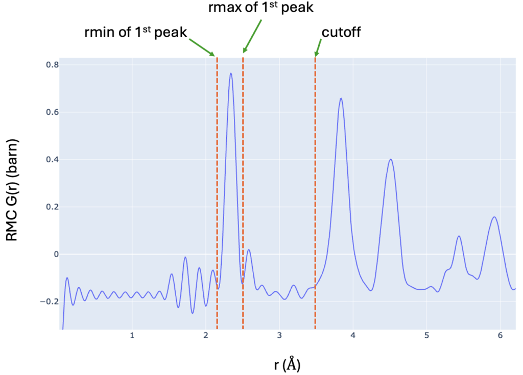
5 1.0 3.0 # cutoff, rmin of 1st peak, rmax of 1st peak. The purpose is to remove ripples
# in the low-r region and those between the first and second peak.Using the template provided above, we can fill in information specific to our data and sample, remove all blank lines and comments, and then run the program like,
stog_new < get_stog_input.txtwhere ‘get_stog_input.txt’ is our saved stog input file.
Things to keep in mind are,
1. In line-4 of the input file, we specify the offset and scale for our data which would then rescale our data according to the formula presented in the comments. The end product we are pursuing here is the normalized total scattering structure factor, which, simply put, should go to 1 at high-Q region.
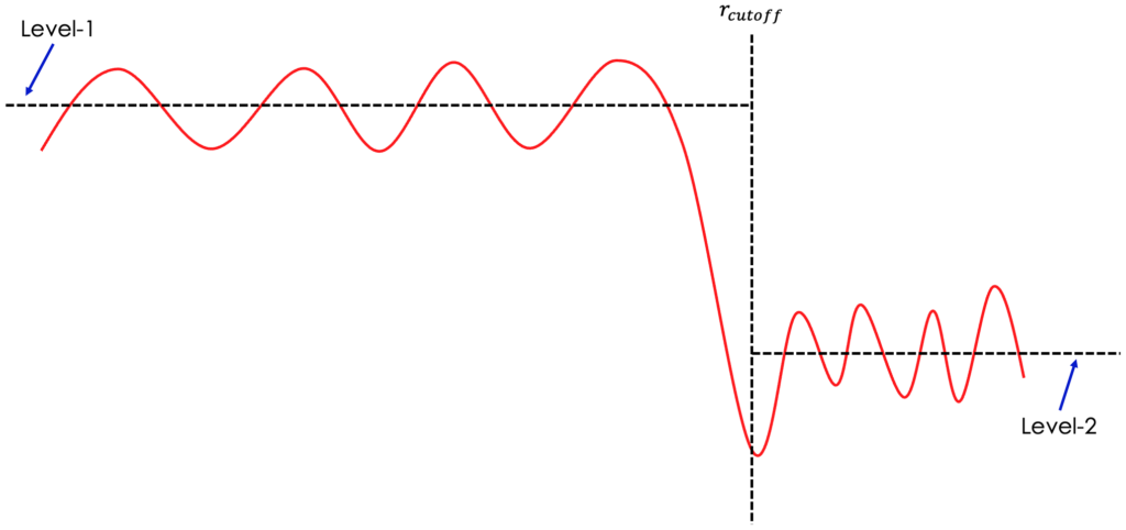
2. However, here may come the question that we have two parameters to control the level at high-Q. In practice, we can have infinite number of combinations of offset and scale to realize the same high-Q behavior. How do we move forward with this? First option is to refer to the low-r behavior in the data output from the Fourier filter step – scale_ft.gr in the example presented above. If the data is scaled properly, we are expecting the Level-1 and Level-2 (see picture down below) to be on the same level.
3. Quite often, even going through the step above still won’t bring our data to absolute scale, in which case the only way left is probably to go through the painful trail-and-error process. That means we may want to play around with different scales of the data and see its effect on the fitting. In most cases, if the data scaling is not proper, not refining scale in RMCProfile has little chance to fit the data well.
4. Alternative option one is to fit scale and offset in RMCProfile, especially for X-ray data.
5. Alternative option two is to fit the scale in, e.g., PDFgui first and use the scale obtained there to rescale our data.
6. For the parameters in the very last line, refer to the following figure for the meaning of ‘cutoff’, ‘rmin of 1st peak’ and ‘rmax of 1st peak’,
Comments
8 responses to “Data pre-processing for RMCProfile”
metoprololo
metoprololo
furosemide 20 mg
furosemide 20 mg
tadalafil daily review
tadalafil daily review
generic sildenafil 100mg
generic sildenafil 100mg
cyclosporine hyperkalemia
cyclosporine hyperkalemia
xenical nz reviews
xenical nz reviews
viagra brazil
viagra brazil
bupropion hcl anxiety
bupropion hcl anxiety